How to create a betting model using expected goals data

Preface

This post was only ever intended to be a brief summary but has ultimately turned into a story of my journey with the betting model interwoven. It’s ended up at over 6,000 words and is an open article of my inspirations, data sources and formulas used. The purpose is to cover everything needed for a like-minded individual to start on their own journey, so here goes…

Introduction to me

With the lockdown resulting in a temporary shutout of many sports, it has provided me with an opportunity for reflection, development and knowledge sharing – the aim of this blog post.

Search Twitter nowadays and there are an abundance of football analysts, some successfully making a living out of it and some who do it for the love it. I lack a scouting or coaching background and have a perception that the industry is difficult to crack so a year or two ago I started on a different path to see if I could use expected goals data to create a betting model.

First and foremost I’m a sports fan. I’ve always been interested in numbers and as I have become older this has naturally progressed into a fascination of data. With an abundance of resources available nowadays I’ve spent many hours manually collating and creating spreadsheets looking for interesting trends and patterns generally to help make predictions, sometimes with a financial investment attached.

I like to think I have a rough grasp of odds offered by bookmakers, be it a good price or a bad price. I’ve never been one to do an accumulator with several odds-on favourites at home, inevitably it would be let down by at least one and didn’t feel like great value, but I had no way of telling.

Moneyball and Mayhew

For a sports fan who loves data, the 2011 film Moneyball about the world of Baseball and advanced analytics would have seemed like a natural fit but I’ll be honest and say I don’t think it even registered on my radar. It wasn’t until 2017 that I can remember first watching the film with one particular scene lodging firming in my memory. 

For those who haven’t seen the film, the scene revolves around the Oakland Athletics general manager Billy Beane played by Brad Pitt. The problem facing them summarised in one simple quote:

“There are rich teams, and there are poor teams. Then there’s 50 feet of crap. And then there’s us”

Billy Beane

With a limited budget available, Beane brings in assistant general manager Paul DePodesta to help build a roster of players using new sophisticated analytical metrics to identify undervalued talent often against the advice of the experienced traditional scout. If you haven’t watched and you think you may be like minded then watch the film, it’s highly recommended and is the inspiration for my journey.

I hadn’t the first idea about Baseball but assumed that something must be transferable to football. This was when I stumbled across a book by James Tippett called The Football Code: The Science of Predicting the Beautiful Game. It was a great introduction to a new concept to me, expected goals, and the use in the real world at SmartOdds and Brentford through owner Matthew Benham.

For those not familiar with expected goals (or xG for short) it is a metric to monitor the quality of a goalscoring chance. A value between 0 and 1 is assigned based on the probability the chance will result in a goal. A 1 in 20 long range shot will have a probability of 5% (an xG of 0.05) whereas a penalty roughly has a 3 in 4 expectancy and therefore an xG of 0.75.

Inspired by the idea of a new advanced metric I searched and read any related article I could find. It was at this point my searches led me to Ben Mayhew, who through his Twitter profile @experimental361, was creating data visualisations using expected goals data.

His website, www.experimential361.com, is full of great content and my interest was piqued further with the match xG timelines. Using a couple of recent examples from matches just before the lockdown in March shows how useful they are to provide a quick snapshot of how a match unfolded.

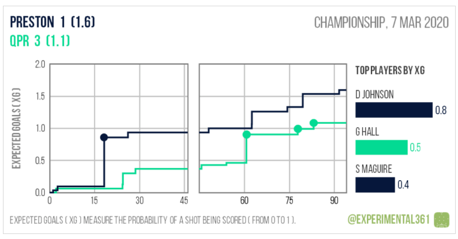
Firstly, a match between Preston North End and Queens Park Rangers could be summarised as: Preston scoring with their first real good chance with little happening in the subsequent 40 minutes. QPR equalised with their best chance of the match but were somewhat fortunate to win the game from thereafter with Preston creating the better chances.

QPR scored 3 goals but were expected to score 1.1 whereas Preston scored 1 goal but were expected to score 1.6. These are the type of games where a 1-1 draw or 2-1 home win would have felt a fairer representation to me based on the chances but also how the game panned out.

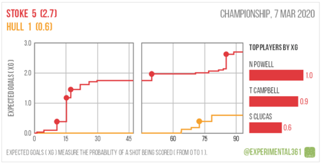
The match between Stoke City and Hull City is more straightforward in that Stoke were totally dominant from the start but are arguably flattered by the scoreline with the hosts scoring 5 goals but were expected to score 2.7.

Intrigued to find out more and keen to have a play around with some new data I wondered if it was possible to create expected goals myself and so I reached out to Ben to support.

Finding Data

I can’t remember whether I was expecting to receive a reply from Ben, and although he understandably didn’t share all his secrets, it was enough information to point me in the right direction and provide motivation to dive right in.

I wasn’t looking to invest financially into any data so it was important that the data was free, consistent and easily accessible. Those who follow the live text commentary from BBC Sport or Sky Sports website will notice that they are typically uniform in nature. Perfect to extract the information required with the text tending to be in a set format.

Each line of text describes an event that has occurred in the match with a couple of examples below from my preferred source, the SportingLife website.

A goal is typically structured as:

A non-scoring attempt structured as:

By recognising the set structure of the various types of events this can be manipulated through use of formulas in Excel or any other preferred coding language into something more useful:

Minute	Event	Attempt Player	Team	Attempt Type	Shot Location	Shot Placement	Assist Player	Assist Type
19	Goal	Daniel Johnson	Preston North End	Left footed shot	Penalty	Bottom right corner
25	Attempt Missed	Jordan Hugill	Queens Park Rangers	Header	Centre of the Box	Misses to the left	Ryan Manning	Corner

This is obviously just two incidents within one match but collating this for numerous events across numerous leagues across numerous seasons quickly builds a database containing thousands of records.

Not keen to manually copy the information I gathered there must be a smarter way. A quick Google search identified a free software called R which could extract the data needed from the websites in bulk. For a beginner Stack Overflow was a great tool to help me pull the data I needed. The time invested was definitely worthwhile and has saved a lot of time in the long term.

The Expected Goals Model

If you are still reading at this point, thanks! The next section and lynchpin for the whole article is creating the expected goals model. The first step is to have a large database of events, the more the better ideally. As shown in the table previously you can extract numerous data items such as the attempt type, shot location, shot placement and assist type. For my model I use just two pieces of information:

– Attempt Type – namely was the attempt a shot or a header

– Shot Location – where on the pitch was the attempt taken from

Now it’s important at this stage to highlight that the quality of an expected goals model is dependent on the quality of the data used. My model is at the simpler end as it’s using free basic descriptive data. Every other model will use different input data in a different way to calculate an expected goals value for an attempt. This is why values from different providers have different values.

The data I use is suitable for my needs as it is free, easy attainable and allows myself to be in control of the calculation. For those looking to find data, FBref, WhoScored and Infogol are three data suppliers who have more detailed data than mine and are a good source for information.

Anyway back to the data I use. By linking the different attempt type and shot location provides various combinations detailing the attempt. For each of these you will be able to calculate the number of times that attempt combination occurred and how often it resulted in a goal. This is the basis of the expected goals formula:

xG value = The number of goals scored / The number of attempts taken

From my database of around 150,000 attempts and just under 17,000 goals I have the following percentages for each type of attempt and the corresponding expected goals value:

Attempt Type	Attempts	Goals	Goal %	xG Value
Penalty	2869	2158	75.2%	0.752
Shot from Very Close Range	3170	1738	54.8%	0.548
Header from Very Close Range	2536	885	34.9%	0.349
Shot from Side of 6 Yard Box	3098	684	22.1%	0.221
Shot from Centre of Box	29592	5149	17.4%	0.174
Free Kick	2712	395	14.6%	0.146
Header from Side of 6 Yard Box	2624	362	13.8%	0.138
Header from Centre of Box	18270	1566	8.6%	0.086
Shot from Difficult Angle	2576	208	8.1%	0.081
Shot from Side of Box	21876	1527	7.0%	0.070
Shot from Long Range	1930	96	5.0%	0.050
Shot from Outside of Box	54510	1948	3.6%	0.036
Header from Side of Box	1058	30	2.8%	0.028
Header from Outside of Box	79	2	2.5%	0.025
Header from Difficult Angle	282	3	1.1%	0.011

It’s at this point the realisation of how infrequent long range goals are scored may refrain a few from shouting “Shooooot” the next time a player has the ball around 25 yards out.

Once each event has been assigned an expected goals value then the possibilities are endless. You can calculate the expected goals for both teams in any given match, the expected goals a player should have scored over a season or the data I use for my betting model: the expected goals scored and conceded by each team over a rolling seasons period.

There’s no wrong way to measure team strength. I’ve chosen a seasons period as I feel it gives a truer reflection of a team’s ability. Shorter 6/10 game periods are useful context and reflect the latest information more quickly but can be biased due to the fixture strength experienced.

Expected Goals in the Real World

Enough of the theory, Here’s an example of the expected goals data I have calculated, in this instance the final table for the 2018-19 Championship table. An important finding to note is that the spread in expected goals scored (xGF) and expected goals conceded (xGA) is a lot narrower than the actual goals scored and conceded.

The ability of the teams within the league are closer than people think. In most cases the teams at the top are good but overperforming somewhat. Think of it as those teams who seem to win lots of games by a single goal when it probably should have been a draw.

Rank	Team	GF	GA	GD	Pts	xGF	xGA	xGD	xPts	xPts Rank
1	Norwich City	93	57	36	94	80	59	21	75	3
2	Sheffield United	78	41	37	89	76	46	30	80	2
3	Leeds United	73	50	23	83	81	43	38	83	1
4	West Bromwich Albion	87	62	25	80	75	64	11	68	6
5	Aston Villa	82	61	21	76	76	63	13	69	5
6	Derby County	69	54	15	74	59	65	-6	61	16
7	Middlesbrough	49	41	8	73	67	63	5	66	9
8	Bristol City	59	53	6	70	64	62	2	65	11
9	Nottingham Forest	61	54	7	66	61	68	-7	61	17
10	Swansea City	65	62	3	65	71	60	11	67	8
11	Brentford	73	59	14	64	66	54	13	69	4
12	Sheffield Wednesday	60	62	-2	64	58	66	-8	59	18
13	Hull City	66	68	-2	62	60	69	-9	57	20
14	Birmingham City	64	58	6	61	60	59	1	64	12
15	Preston North End	67	67	0	61	61	68	-6	58	19
16	Blackburn Rovers	64	69	-5	60	66	68	-2	62	13
17	Stoke City	45	52	-7	55	54	58	-3	62	15
18	Wigan Athletic	51	64	-13	52	69	70	-1	62	14
19	Queens Park Rangers	53	71	-18	51	66	62	3	66	10
20	Reading	49	66	-17	47	50	85	-35	45	23
21	Millwall	48	64	-16	44	69	60	9	67	7
22	Rotherham United	52	83	-31	40	64	79	-15	55	21
23	Bolton Wanderers	29	78	-49	32	44	70	-26	48	22
24	Ipswich Town	36	77	-41	31	45	82	-37	45	24

Summarising the table above can help identify the following based on the underlying expected goals numbers:

– Sheffield United were the strongest team promoted.

– Leeds United were unlucky not be promoted and were the strongest team remaining in the league.

– Derby County overachieved to reach the playoffs and appear to be of mid-team quality.

– Brentford, Swansea City and almost relegated Millwall were superior to their finishing positions and were of a playoff pushing quality.

– Hull City and Reading were the weakest two teams to remain in the league.

– Rotherham United were the strongest team to be relegated.

Fast forward to this season and it’s striking how many of those have come to realisation. From my experience I have found expected goals to be a much better indicator of future performance than actual goals. This is the main reason why I place some much value in the use of this particular metric.

Expected Points

For those interested in expected points, labelled as xPts in the table, this is an additional metric using expected goals. My method is to look at the difference in expected goals of the two teams for a particular match.

Using one of matches highlighted earlier of Preston North End 1 (1.6) – Queens Park Rangers 3 (1.1), provides a xG difference of +0.5 for Preston and -0.5 for QPR. The next step is to look at how often a team actually wins, draws or loses with this difference and multiplying this by the points earned for each outcome.

This is a simplistic approach as it just looks at the total xG not the number and quality of the individual chances which would impact the xPts. There are calculators available online to plug in the attempts to provide the probability but in absence of doing this in bulk I have devised this methodology.

For example if a team with +0.5 xG difference wins half of the matches, draws 30% of the time and loses the remainder this could be calculated as:

Expected points for a team with +0.5 xG difference

= (Team wins 50% of the time * 3 points for a win) + (Team draws 30% of the time * 1 point for a draw) + (Team loses 20% of the time * 0 points for a loss)

= (50% * 3) + (30% * 1) + (20% * 0)

= 1.8

Expected points for Preston North End would be 1.8.

On the contrary this would mean the team with a -0.5 xG difference would lose half of the matches, draw 30% of the time and win the remainder. This would be calculated as:

Expected points for a team with -0.5 xG difference

= (Team wins 20% of the time * 3 points for a win) + (Team draws 30% of the time * 1 point for a draw) + (Team loses 50% of the time * 0 points for a loss)

= (20% * 3) + (30% * 1) + (50% * 0)

= 0.9

Expected points for Queens Park Rangers would be 0.9.

The combined expected points won’t add up to 3 points as while a win distributes a total of 3 points, drawn games only distribute a total of 2 points.

Due to the nature of the calculations it is best to group together similar values to ensure each banding has significant volume and also helps create a smooth curve to ensure the xPts increases as the xG difference increases.

The table below shows the values I use and show Preston’s xPts to be 1.77 and QPR’s xPts to be 0.95 for the match in question.

xG Difference	xPts Value
>3.20	2.78
>2.70 to 3.20	2.62
>2.10 to 2.70	2.45
>1.50 to 2.10	2.28
>1.00 to 1.50	2.11
>0.75 to 1.00	1.94
>0.45 to 0.75	1.77
>0.30 to 0.45	1.60
>0.00 to 0.30	1.43
>-0.30 to 0.00	1.27
>-0.45 to -0.30	1.11
>-0.75 to -0.45	0.95
>-1.00 to -0.75	0.80
>-1.50 to -1.00	0.66
>-2.10 to -1.50	0.52
>-2.70 to -2.10	0.39
>-3.20 to -2.70	0.26
<= -3.20	0.15

Calculating Score Probabilities

Now the expected goals data are summarised for each team can be used to predict the outcome of a future match. This is done by calculating the average projected goals using a Poisson distribution. A Poisson distribution is used as the shape of the distribution closely follows the distribution of goals scored in football matches. For those looking for a little bit more detail then the article written below on the Pinnacle website is helpful.

https://www.pinnacle.com/en/betting-articles/Soccer/how-to-calculate-poisson-distribution/MD62MLXUMKMXZ6A8

To demonstrate the calculation for a match I will use my version of the 2018-19 Championship table shown earlier in the article to project the outcome of a fictional match between Preston North End and QPR assumed to be on the first day of the 2019-20 Championship season.

The first step is to calculate the average expected goals scored and expected goals conceded for the Championship. Across the whole season there were 1542 expected goals according to my model (1473 actual goals scored), 857 expected for the home team (836 actual) and 686 expected for the away team (637 actual) with the 24 championship teams playing 23 times at home (552 home teams in total) and 23 times away from home (552 away teams in total). These numbers can be used to calculate a number of formulas.

Average expected goals scored by the home team = 857 / 552 = 1.55 goals per match

Average expected goals conceded by the home team = 686 / 552 = 1.24 goals per match

Average expected goals scored by the away team = 686 / 552 = 1.24 goals per match

Average expected goals conceded by the away team = 857 / 552 = 1.55 goals per match

To calculate the values for specific teams we need the expected goals data split by home and away performance. My data for the 2018-19 Championship table is shown below with values at 2 decimal places.

Team	HxGF	HxGA	HxPts	AxGF	AxGA	AxPts
Aston Villa	44.45	30.81	38.67	31.44	32.13	30.59
Birmingham City	32.74	25.01	35.85	27.66	34.07	28.10
Blackburn Rovers	37.15	28.33	35.78	29.16	39.74	26.57
Bolton Wanderers	21.44	31.75	25.11	22.56	37.87	22.83
Brentford	40.53	22.16	41.16	25.65	31.34	28.31
Bristol City	32.46	25.26	35.70	31.15	36.48	28.86
Derby County	34.68	24.22	37.61	23.89	40.54	23.23
Hull City	32.55	29.50	32.76	27.17	39.68	23.84
Ipswich Town	25.63	39.12	24.82	19.77	43.07	19.72
Leeds United	46.04	21.80	44.62	34.80	21.48	38.27
Middlesbrough	39.28	29.37	37.20	27.90	33.30	28.91
Millwall	35.98	27.05	36.95	32.90	33.17	30.18
Norwich City	42.03	23.78	42.02	38.10	35.20	32.98
Nottingham Forest	33.61	29.22	34.56	27.46	38.73	26.18
Preston North End	36.79	32.23	33.22	24.40	35.37	24.55
Queens Park Rangers	38.05	27.92	37.06	27.68	34.43	28.88
Reading	24.23	36.76	25.42	25.36	48.00	19.66
Rotherham United	37.41	40.45	29.76	26.56	38.18	24.99
Sheffield United	37.53	20.73	40.78	38.83	25.37	38.79
Sheffield Wednesday	33.36	29.46	33.73	24.99	37.03	24.78
Stoke City	29.39	24.00	34.75	25.06	33.92	27.28
Swansea City	41.49	27.18	38.34	29.16	32.83	28.64
West Bromwich Albion	44.73	29.42	39.59	30.69	34.93	28.48
Wigan Athletic	35.19	30.19	33.71	33.38	39.86	28.32
League Total	857	686		686	857
League Average	35.70	28.57		28.57	35.70
Match Average	1.55	1.24		1.24	1.55

In the hypothetical example of Preston North End v QPR we will need to calculate the average expected goals specific to both teams by assessing their attacking strength, the opponent’s defending strength and league average performance using the following formulas:

Preston’s average expected goals at home to QPR

= Preston’s home attacking strength x QPR’s away defending strength x average home goals scored

Preston’s home attacking strength

= Preston’s HxGF / League Average HxGF

= 36.79 / 35.70

= 1.031

Anything over 1 implies better than the league average, or in this case Preston are expected to score 3.1% more at home than an average Championship team

QPR’s away defending strength

= QPR’s AxGA / League Average AxGA

= 34.43 / 35.70

= 0.964

Anything under 1 implies better than the league average, or in this case QPR are expected to concede 3.6% fewer away than an average Championship team

Preston’s average expected goals at home to QPR

= Preston’s home attacking strength x QPR’s away defending strength x average home goals scored

= 1.031 x 0.964 x 1.55

= 1.543

QPR’s average expected goals away to Preston

= QPR’s away attacking strength x Preston’s home defending strength x average away goals scored

QPR’s away attacking strength

= QPR’s AxGF / League Average AxGF

= 27.68 / 28.57

= 0.969

Anything over 1 implies better than the league average, or in this case QPR are expected to score 3.1% fewer away than an average Championship team

Preston’s home defending strength

= Preston’s HxGA / League Average HxGA

= 32.23 / 28.57

= 1.128

Anything under 1 implies better than the league average, or in this case Preston are expected to concede 12.8% more away than an average Championship team

QPR’s average expected goals away to Preston

= QPR’s away attacking strength x Preston’s home defending strength x average away goals scored

= 0.969 x 1.128 x 1.24

= 1.351

To conclude we would expect the average scoreline to be:

Preston North End 1.543 – Queens Park Rangers 1.351

Obviously teams do not score a decimal amount of goals therefore we need to distribute this average using Excel’s Poisson formula. The formula is structured in the form of

= POISSON(x, mean, cumulative)

You can calculate the probability the team scores a specific amount of goals by replacing the x with the number of goals, replacing the mean with the average expected goals calculated above and setting cumulative to false.

For example, the probability of Preston scoring 0 goals at home to QPR can be calculated as:

=POISSON(0, 1.543, FALSE)

=0.214

=21.4%

Repeating this for both teams up to 5 goals will produce the following values

Team	0	1	2	3	4	5
Preston North End	21.4%	33.0%	25.4%	13.1%	5.0%	1.5%
Queens Park Rangers	25.8%	34.9%	23.7%	10.7%	3.6%	1.0%

Calculating Match Probabilities

My model assumes that goals are scored independently of each other and therefore the probability of specific scorelines can be calculated by multiplying the two scores together. A 0-0 scoreline would have a probability of 5.5% (21.4% x 25.8%) whereas a 1-1 will have a probability of 11.5% (33.0% x 34.9%).

Calculating the probability of a Preston win is simply a case of adding together all of the favourable scorelines (1-0, 2-0, 2-1, 3-0, 3-1, 3-2 etc.) which comes out as 41.8%. The probability of any draw is 24.7% and a QPR win is 33.5%.

Armed with probabilities for the theoretical match, the next step is to compare these with the bookmakers odds to highlight if there are any differences and by how much. Bookmakers odds are traditionally either shown as fractions or decimals and some hypothetical odds for the match would be shown as the following.

Fractional Odds

Preston North End	Draw	Queens Park Rangers
11/10	5/2	11/4

Decimal Odds

Preston North End	Draw	Queens Park Rangers
2.1	3.5	3.75

To be able to assess where the model differs from the bookmakers odds it is important to convert the odds back to probabilities. This can be done using the following formulas for either of the odds to calculate the probabilities.

Match Outcome	Fractional Odds	Formula	Decimal Odds	Formula	Probability
Preston North End	11/10	=10/(11+10)	2.1	=1/2.1	47.6%
Draw	5/2	=2/(5+2)	3.5	=1/3.5	28.6%
Queens Park Rangers	11/4	=4/(11+4)	3.75	=1/3.75	26.7%

You may have noted that the bookmakers probabilities total more than 100%, or 102.9% in this case. This is called the overround and is always above 100% to ensure the bookmakers make an overall profit on the match assuming they are able to obtain a fair split of bets across the various outcomes according to the probabilities.

With the odds shown in probabilities this can then be compared to the probabilities from the expected goals model to see where there are any discrepancies.

Match Outcome	Modelled Probability	Bookmakers Probability	Difference
Preston North End	41.8%	47.6%	-5.8%
Draw	24.7%	28.6%	-3.9%
Queens Park Rangers	33.5%	26.7%	+6.8%

Both the model and the bookmakers believe the most likely outcome is a Preston North End win but the bookmakers believe it is more likely to occur than the model. A Queens Park Rangers win is the only outcome the model estimates to be more likely than the bookmakers, and although the likelihood is lower than Preston win, this would be the value selection to make in this scenario.

To highlight why it is the selection think of the scenario as a roll of a fair dice where you could bet on the following outcomes: 1, 2 or 3; 4 or 5; and 6. We know each individual numbers are equally likely to appear so betting on the outcome should be solely based on the odds offered.

Outcome	Modelled Probability	Bookmakers Odds (and Probability)	Difference
1, 2 or 3	50.0%	4/5 (55.5%)	-5.5%
4 or 5	33.3%	9/4 (30.7%)	+2.6%
6	16.6%	4/1 (20.0%)	-3.4%

We all know that a 1, 2 or 3 is the most likely outcome but the odds available represent poor value and so over time we should expect to lose money betting on this outcome. It is important to recognise we are not expected to win every bet but ensure we are betting on outcomes that are more likely to occur than the bookmakers odds suggest, as highlighted by a positive difference value.

Staking Strategy

Once we have identified the bets to place, a Queens Park Rangers win in the hypothetical example, the final step is to place the bets.

The last inspiration was to read a book by Joe Peta called “Trading Bases: How a Wall Street Trader Made a Fortune Betting on Baseball”. The title is a perfect synopsis of the book but one of the useful sections highlights how a bigger stake should be placed on bets with a bigger difference between the modelled probability and bookmakers probability, the margin. The logic makes perfect sense in that the bigger the perceived error in the bookmakers odds the bigger the stake should be to capitalise on it.

My staking place roughly follows the approach he adopted in the book and is detailed in the table below.

Margin between Modelled Probability and Bookmaker Probability	% of Bank Staked	Stake for a 100pt Bank
>15 %	2.0%	2pt
>13-15 %	1.5%	1.5pt
>11-13 %	1.0%	1pt
>9-11 %	0.5%	0.5pt
>6-9 %	0.4%	0.4pt
>3-6 %	0.2%	0.2pt

The hypothetical bet on Queens Park Rangers with a +6.8% margin means the selection would have been a 0.4pt win. For the dice roll, the margin of +2.6% would not have met the minimum threshold I use of 3%.

Paper Trading

This now brings the story up to the start of the 2019/20 season where I thought it would be a good idea to paper trade the selections (i.e. record the outcome of the selections identified but with no bets placed) to assess the volume of bets selected, outcome of the bets and the time needed to follow the model.

The first stumbling block was how to assess promoted/relegated teams in terms of their expected goals quality. Obviously using the expected goals from the Championship table for Rotherham United, Bolton Wanderers and Ipswich Town, the three relegated teams, in the League One fixtures would have underestimated their actual quality as their values were achieved against a higher calibre of opposition.

The only sensible and suitable solution I could see was to use cup fixtures between different leagues to estimate the adjustments required for promoted and relegated teams. Obviously teams at not always at full strength but the numbers provided gave an appropriate outcome.

Essentially this means that relegated teams had their xGF increased and xGA reduced to estimate what this performance would have equated to if playing in the division below. The reverse of this is done for promoted teams.

Promoted Teams

Previous Season League	Next Season League	Home xGF Adjustment	Home xGA Adjustment	Away xGF Adjustment	Away xGA Adjustment
Championship	Premier League	x 0.704	x 1.426	x 0.713	x 1.467
League One	Championship	x 0.764	x 1.389	x 0.761	x 1.433
League Two	League One	x 0.815	x 1.296	x 0.815	x 1.259

Relegated Teams

Previous Season League	Next Season League	Home xGF Adjustment	Home xGA Adjustment	Away xGF Adjustment	Away xGA Adjustment
Premier League	Championship	x 1.411	x 0.702	x 1.403	x 0.677
Championship	League One	x 1.296	x 0.705	x 1.287	x 0.691
League One	League Two	x 1.236	x 0.779	x 1.239	x 0.800

The numbers show that there is a bigger difference between leagues the higher the pyramid you go. An example of how this is applied for one of the relegated teams, Rotherham United, is shown below:

Scenario	HxGF	HxGA	AxGF	AxGA	Performance
2018-19 Championship Performance	37.41	40.45	26.56	38.18	21st in Championship
2018-19 Championship Performance Adjusted to League One Standard	48.48 (37.41 x 1.296)	28.52 (40.45 x 0.705)	34.28 (26.56 x 1.287)	26.38 (38.18 x 0.691)	3rd in League One (or 1st with Luton and Barnsley promoted)

This adjustment calculated Rotherham United to be the strongest team in League One for the following season aided by the fact the two teams of a higher standard, Luton Town and Barnsley, were both promoted to the Championship. Ipswich Town and Bolton Wanderers were equivalent to mid table teams in League One.

It’s also important to highlight that I use a rolling seasons data for the calculation of the teams strength so it is a case of replacing the oldest game in the 46 game period with the new one each game week to ensure the data was always up to date.

The additional adjustments caused a slight delay meaning paper trading didn’t actual begin until October 2019 and here are my results to date…

Is it Successful?

The first factor I found is that the model throws up a lot of selections. Across the top four leagues in England the model was highlighting a selection for 60% of the matches. So a typical full weekend schedule of 10 Premier League matches, 12 Championship matches, 11 League One matches (due to no Bury) and 12 League Two matches would highlight around 25-30 teams to bet on. A lot more than I was expecting.

Secondly, the model didn’t select odds on selections very often. This inevitably meant the model fancied outsiders which made sense as I had often read that favourites are typically underpriced due to their popularity in the Saturday accumulators. This meant the strike rate would be lower than expected and that I would need a constant supply of odds against selections to win to ensure it remained profitable.

Five and a half months in and the model is indeed showing a profit. From a starting bank of 100 points it would now stand at 120.64 points at the point of lockdown. One detail that has surprised me is the consistency of the results.

All individual months have shown a profit bar one and the amount has been roughly the same aided somewhat due to a fairly uniform win percentage.

Bet History by Month

Date	Total Games	Bets	Bets %	Wins	Wins %	Stake	Return	Profit	ROI	Bank
Oct-19	195	133	68%	46	35%	62.50	67.58	5.08	8%	105.08
Nov-19	166	111	67%	36	32%	62.10	61.56	-0.54	-1%	104.54
Dec-19	243	141	58%	46	33%	80.90	84.43	3.53	4%	108.08
Jan-20	216	126	58%	40	32%	60.60	65.92	5.32	9%	113.39
Feb-20	265	160	60%	49	31%	79.20	84.29	5.09	6%	118.49
Mar-20	69	43	62%	11	26%	23.70	25.86	2.16	9%	120.64
Total	1199	714	60%	228	32%	369.00	389.64	20.64	6%

Now this still feels like a small sample and is only really half a season so I’m not sure if this is down to luck, expected goals data not fully factored into bookmaker odds yet or a combination of the two. I’m not entirely sure at what point I will know if this is not luck (perhaps someone reading will be able to help) but I know nobody likes to follow a losing model for too long at too much of an expense.

To provide further context of the results to date:

Bet History by League

– League Two has the highest strike rate but is the only league not to make a profit.

– The Premier League has the lowest strike rate and minimal profit. The league probably the most wagered on in the world, particularly with large syndicates, and therefore the odds should be the most accurate and toughest to profit from.

League	Total Games	Bets Made	Bets Made %	Wins	Wins %	Stake	Return	Profit	ROI
Premier League	239	155	65%	42	27%	84.00	85.28	1.27	2%
Championship	360	227	63%	68	30%	128.70	141.56	12.86	10%
League One	292	160	55%	52	33%	73.70	86.26	12.56	17%
League Two	312	174	56%	67	39%	83.20	76.92	-6.28	-8%
Total	1203	716	60%	229	32%	369.60	390.01	20.41	6%

Bet History by Result

– Away wins are by far the most profitable outcome for the model. This reiterates the initial idea with outsiders tending to be the away team with home teams often over bet and providing poor value

– The model very rarely selects a draw

Result	Bets Made	Wins	Wins %	Stake	Return	Profit	ROI
Home	389	143	37%	216.10	192.62	-23.48	-11%
Draw	12	2	17%	3.30	3.95	0.65	20%
Away	315	84	27%	150.20	193.44	43.24	29%
Total	716	229	32%	369.60	390.01	20.41	6%

Bet History by Model Percentage

– A rough correlation between the modelled percentage and the win percentage but surprising low for the most likely outcomes.

– The 20%-50% modelled probability section the most successful for profits.

Model Percentage	Bets Made	Wins	Wins %	Stake	Return	Profit	ROI
70%+	9	4	44%	6.20	4.65	-1.55	-25%
60-70%	39	23	59%	35.70	41.31	5.61	16%
50-60%	120	50	42%	81.20	66.56	-14.64	-18%
40-50%	192	75	39%	101.40	110.50	9.10	9%
30-40%	177	47	27%	83.60	80.32	-3.28	-4%
20-30%	141	25	18%	51.10	74.76	23.66	46%
10-20%	38	5	13%	10.40	11.90	1.50	14%
0-10%	0	0	0%	0.00	0.00	0.00
Total	716	229	32%	369.60	390.01	20.41	6%

Bet History by Odds

– Odds on selections are rarely highlighted but do turn a slight profit

– The model is profitable for any selection priced at 6/4 or higher with strong crossover from the Away win population.

Odds	Bets Made	Wins	Wins %	Stake	Return	Profit	ROI
Odds On	53	31	58%	20.20	22.12	1.92	10%
Evens – <6/4	142	56	39%	85.00	69.56	-15.45	-18%
6/4 – <2/1	128	55	43%	61.80	75.03	13.23	21%
2/1 – <3/1	158	50	32%	88.40	104.14	15.74	18%
3/1+	235	37	16%	114.20	119.17	4.97	4%
Total	716	229	32%	369.60	390.01	20.41	6%

Bet History by Stake

– Probably the most important one to consider. Disappointingly the selections with the biggest margin, and therefore biggest stake, have a low strike rate and return a loss.

– Beyond that and it shows the benefit of the staking strategy. The second most confident bucket provide a large profit with the lowest confident bucket the only other one providing a loss.

– Interesting to highlight that a flat staking plan would have shown a loss.

% of Bank Staked	Bets Made	Wins	Wins %	Stake	Return	Profit	ROI
2.0%	39	11	28%	78.00	67.70	-10.30	-13%
1.5%	35	16	46%	52.50	83.45	30.95	59%
1.0%	49	15	31%	49.00	49.95	0.95	2%
0.5%	105	39	37%	52.50	56.02	3.52	7%
0.4%	200	62	31%	80.00	80.86	0.86	1%
0.2%	288	86	30%	57.60	52.04	-5.56	-10%
Total	716	229	32%	369.60	390.01	20.41	6%

What’s Next?

The next step was to finish paper trading for this season and then to to start financial investing in the model for the 2021/22 football season. Unfortunately the Coronavirus has played havoc with that and with matches being behind closed doors it is unknown how home advantage will be affected. The model is built on data with football played under circumstances so betting on games with no fans seems unsuitable. It will be interesting to see how home advantage is impacted for the remaining games this season to help direct the plan for next season.

That’s everything. Over 6,000 words and numerous tables/formulas. It’s an article a younger me would have loved to read at the start of my journey. I hope someone has managed to get to the end and found it enjoyable, helpful or mildly interesting.